PCA, K-means, and pLSA (数理情報工学演習第二A)
Hand out and assignments. Assignments are due
Wednesday, July 17.
Principal Component Analysis
United States Postal Service (USPS) Data
Load the data
			data=importdata('data/elem/usps/zip.train');
			Y=data(:,1);
			X=data(:,2:end)';
Visualize some of the training examples
			for ii=1:10
			subplot(1,10,ii); imagesc(reshape(X(:,ii),[16,16])'); colormap gray; title(int2str(Y(ii)));
			end
Subtract mean image
			xm=mean(X,2);
			Xb = bsxfun(@minus, X, xm);
Compute PCA
[U,S,V]=svd(Xb);
Use Mark Tygert's
pca.m if this takes too much time.
[U,Lmd,V]=pca(Xb, 50, 10); % obtain the 50 largest singular values/vectors
Visualize the singular-value spectrum
figure, plot(diag(S),'-x')
Question: Given singular-values $s_1,s_2,...s_p$ (p is the number of dimensions 256), what fraction of the total variance is explained if we truncate the SVD at the $k$th singular-values/vectors?
Visualize the principal components
			for ii=1:50
			subplot(5,10,ii); imagesc(reshape(U(:,ii),[16,16])'); colormap gray;
			end
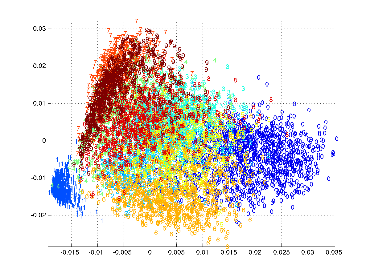
Visualize the top two-dimensional projection
			figure;
			colormap jet; col=colormap;
			for cc=1:10
			ix=find(Y==(cc-1));
			text(V(ix,1), V(ix,2),int2str(cc-1), 'color', col(ceil(size(col,1)*cc/10),:));
			end
			xlim([min(V(:,1)), max(V(:,1))]); ylim([min(V(:,2)),max(V(:,2))]);
Advanced: Face images
How to read the data
I=imread('att_faces/s1/1.pgm');
k-means Clustering
Use the same USPS data set.
Implement k-means clustering
- Download the skeleton: kmeans.m.
- Implement the "cluster center update step".
- Implement the "cluster assignment update step".
Run k-means
With the number of clusters 10:
[M,Z] = kmeans(X, 10);
Visualize the cluster centers
			for ii=1:10
			subplot(1,10,ii); imagesc(reshape(M(:,ii),[16,16])'); colormap gray;
			end
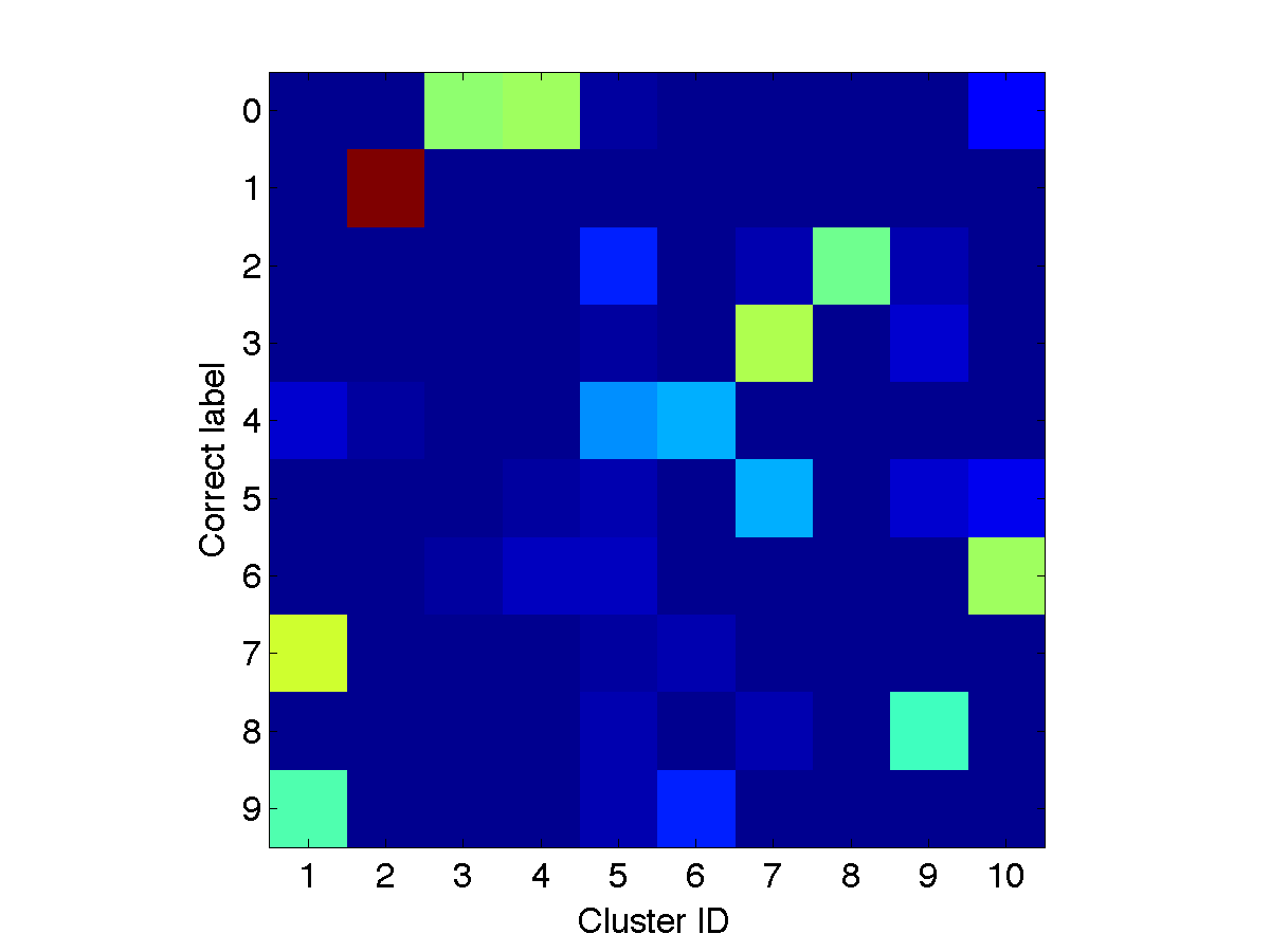
Check whether the cluster assignments are consistent with the class labels
Download a function
loss_confusionMatrix.m to compute the confusion matrix and
			[Yout, JJ, NN]=find(Z);
			C=loss_confusionMatrix(Y, Yout)
			figure, imagesc(C); set(gca,'yticklabel',0:9);
Probabilistic Latent Semantic Indexing (pLSA)
20 Newsgroups data set
Read the data
Read the vocabulary
			voc=importdata('vocabulary.txt');
			D=length(voc);
Read the labels and data
			Y=load('matlab/train.label');
			N=length(Y);
			load('matlab/train.data');
			X=sparse(train(:,2),train(:,1),train(:,3),D,N);
Remove stop words
Download
findsubset.m
			stop=importdata('stopwords.txt');
			I=findsubset(voc, stop); I=I(~isnan(I));
			X(I,:)=[];
			voc(I)=[];
Implement pLSA
- Download the skeleton plsa_em.m.
- Implement the E-step.
- Implement the M-step.
Run pLSA
With the number of topics 20
			K=20;
			[Phi,Pi,nlogP]=plsa_em(X,K,200);
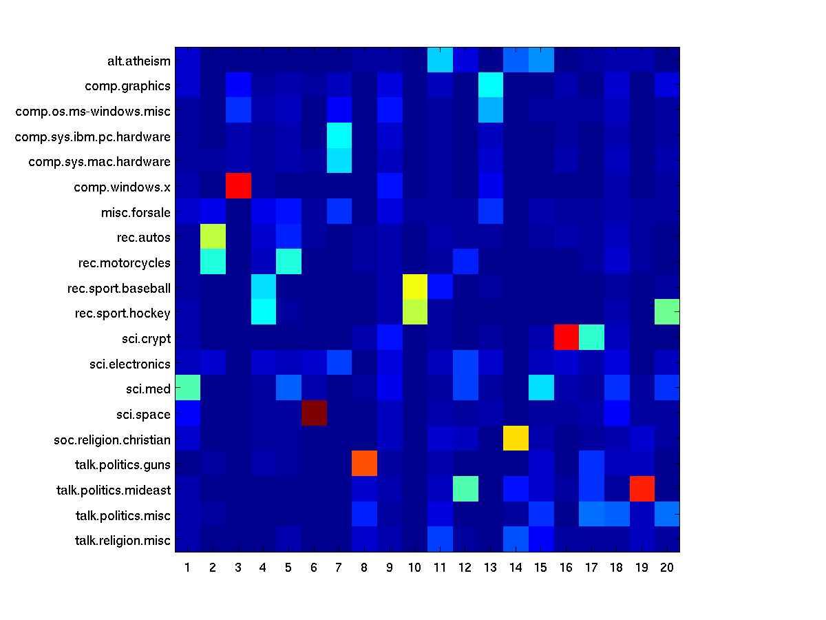
Assess the coherence between the true class labels
			top20=cell(20,K);
			for ii=1:K
			[ss,ix]=sort(-Phi(:,ii)); top20(:,ii)=voc(ix(1:20));
			end
Assess the coherence between the true class labels
Calculate the probability of labels given a topic P(y|c)(y: class label, c: topic)
			Pyc=zeros(20,K);
			for cc=1:20
			Pyc(cc,:)=sum(Pi(:,Y==cc)');
			end
			Pyc=bsxfun(@rdivide, Pyc, sum(Pyc));
			figure, imagesc(Pyc);
			tmp=importdata('matlab/train.map');
			set(gca,'ytick',1:20,'yticklabel',tmp.textdata)
References